Are you tired of spending several hours in Excel to perform repetitive tasks and wish that there could be hacks to do the same operation in a matter of a few seconds? Then, we have good news for you!
Excel offers different smart hacks or tricks that can turn it from a time-draining tool into a time-saving application. So, stay tuned as in this guide, we will discuss the top Excel hacks that can save your hours of work.
1. Combine Multiple Cells into One Cell
Within your Excel data, you can merge or combine the values of multiple cells into a single one using various methods depending on your specific requirements. The most common way to combine cells is to use the & operator.
This operator is very useful when you want to create a single field, such as a full name, by combining data from separate columns. Here’s how to do it.
- Select the cell where you want the combined text to appear in your Excel sheet.
- Type
=to start a formula. - Select the first cell you want to combine.
- Enter
&(the ampersand symbol). - Select the second cell you want to combine.
- Press Enter.
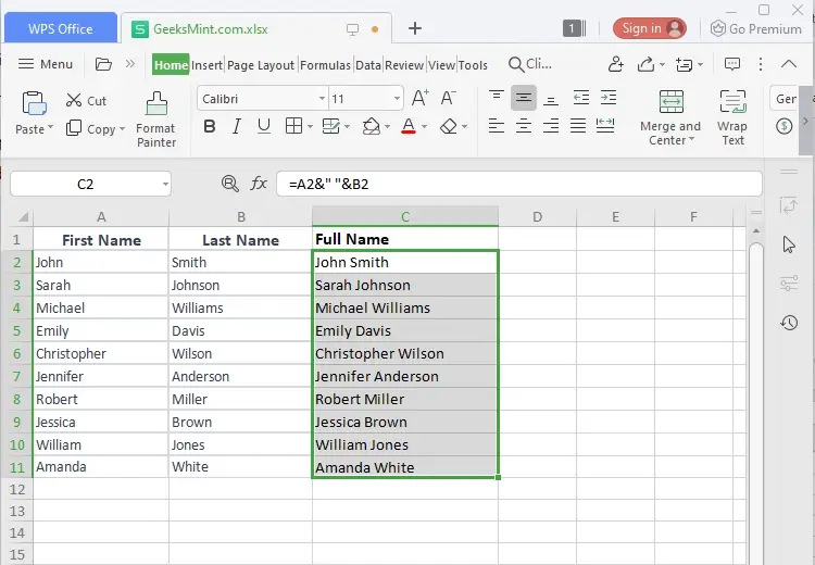
In our case, we want to combine or merge the “First Name” and “Last Name” in the third column named “Full Name“. To do so, we will type the provided formula
=A2&" "&B2
The above formula uses the ampersand “&” operator for combining the contents of cells A2 and B2 with a space between them:
2. Using SEQUENCE() Function
The SEQUENCE() function generates or produces a sequence of numbers in Excel such as a series of consecutive integers, in a column or row. This function is helpful for creating lists of numbers or a series of values that follow a specific pattern or sequence.
The SEQUENCE function has the following syntax:
=SEQUENCE(rows, columns, starting_number, step)
Where
- Rows: The number of rows you want in the sequence.
- Columns: The number of columns you want in the sequence. If you have not provided it, it defaults to 1 column.
- Start: The starting value or number of the sequence. If not provided, it defaults to 1.
- Step: The increment between each value in the sequence. If not provided, it defaults to 1.
Here’s an example of how to use the SEQUENCE function:
To use the SEQUENCE() function, move to the cell where you want the sequence to begin. For instance, in the A1 cell, we will enter the following formula:
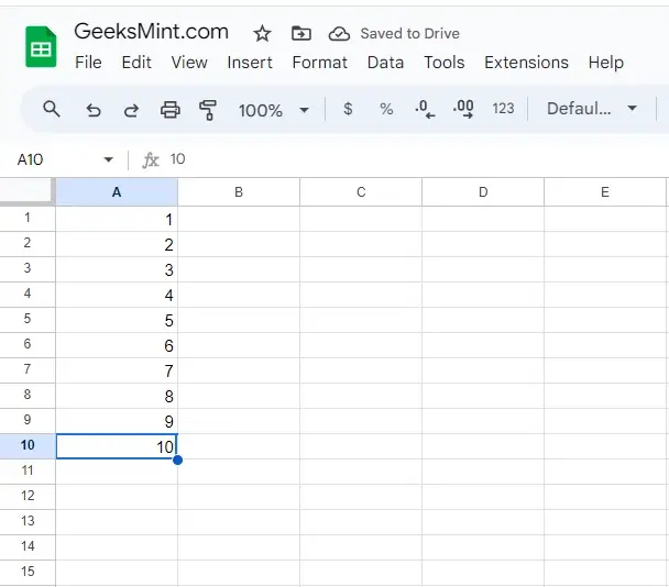
=SEQUENCE(10)
In the above formula, the number “10” indicates that we want a sequence of 10 numbers. Note that you can set this value as per your requirements:
Then, hit the “Enter” key. This will generate a column of numbers from 1 to 10 in a single column.
If you want to create a horizontal sequence, you can specify the number of rows and columns as follows:
=SEQUENCE(1, 10)
This will generate a row of numbers from 1 to 10 in a single row.
You can also specify a different starting value and step size. For example:
=SEQUENCE(5, 1, 10, 2)
Here the function will generate a column of numbers starting from 10 and incrementing by 2, resulting in the values 10, 12, 14, 16, and 18 in a single column.
3. Using SUBSTITUTE() Function
The SUBSTITUTE() function replaces or substitutes the defined substring within a text string with another substring.
The syntax is as follows:
=SUBSTITUTE(text, old_txt, new_txt, [instance_num])
SUBSTITUTE() replaces instances of old_txt with new_txt in a text string. You can also specify [instance_num] for controlling which occurrence of old_txt is needed to be replaced.
Here is an example of how to use the SUBSTITUTE function:
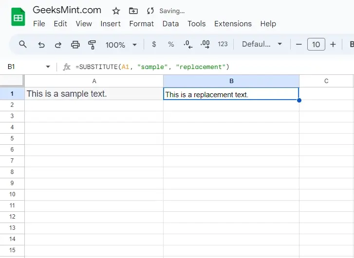
To use the SUBSTITUTE() function, open the Excel file that holds your desired data. For example, cell A1 has a text string “This is a sample text“.
Specify the below-provided formula in the cell where it is needed to add the modified text:
=SUBSTITUTE(A1, "sample", "replacement")
The above formula replaces the word “sample” with “replacement” in the text of the selected cell:
4. Using COUNTIF() Function
COUNTIF() function is one of the powerful and commonly used functions to count the occurrences or number of cells within a range that fulfills the given criteria. It is basically used for data analysis and creating summary reports.
The syntax of the COUNTIF function is as follows:
=COUNTIF(range, criteria)
Where
- Range: This is the range of cells you want to count.
- Criteria: This is the condition or criteria you want to apply to the range.
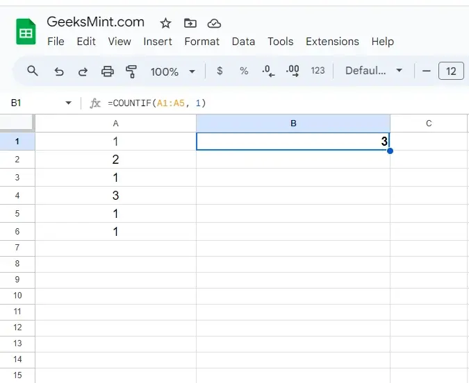
For the purpose of using the COUNTIF() function, enter your data in a column. For example in cells A1 to A6, we will enter the numbers like 1, 2, 1, 1, 3, 1, 1.
Then, in another cell, specify the COUNTIF formula for counting the occurrences of a specific number such as 1 in the range A1 to A5 cells:
=COUNTIF(A1:45, 1)
As a result, Excel will return the count of the given number which would be 3 in this scenario:
5. Using DAYS() Function
The DAYS() function calculates the difference or number of days between the specified two dates.
The syntax of the DAYS() function is as follows:
=DAYS(end_date, start_date)
Where
- end_date: is the later date.
- start_date: is the earlier date
The DAYS() function evaluates the difference between the end_date and start_date.
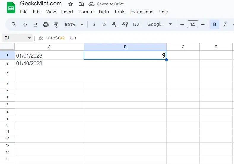
For instance, in one cell, enter the start date as “01/01/2023” and in another cell, enter “01/10/2023” as the end date. Next, in the third cell, specify the below-given formula for calculating the difference between these two dates:
=DAYS(A1, A2)
Consequently, “9” will be displayed as the difference between both dates in the selected cell:
6. Using XLOOKUP() Function
The XLOOKUP() function is a powerful and versatile lookup tool designed to replace and enhance the capabilities of functions like VLOOKUP, and HLOOKUP function.
This function is designed to find and retrieve the value in the defined range or a table and outputs a respective value from another range.
The syntax of the XLOOKUP() function:
=XLOOKUP(lookup_value, lookup_array, return_array, [if_not_found])
XLOOKUP() searches for a value in a lookup_array and outputs a corresponding value from the return_array. You can also specify [if_not_found] to control what to show in the cell if no match is found.
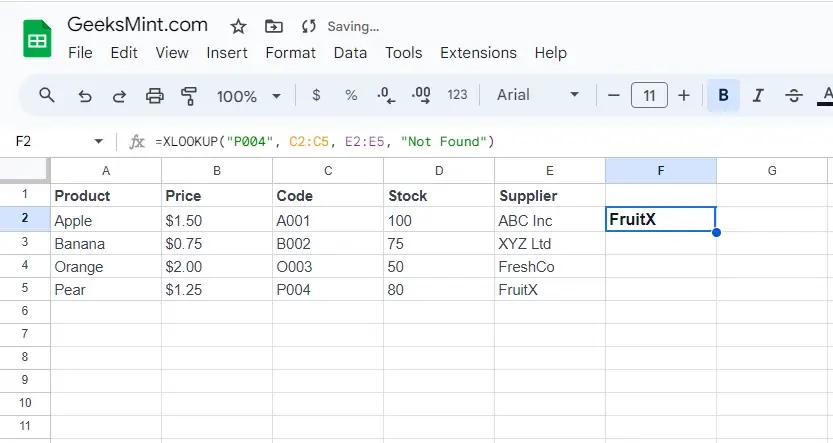
For instance, we want to find the supplier of the product having the code “P004“. To do so, we will enter the below-given formula:
=XLOOKUP("P004", C2:C5, E2:E5, "Not Found")
Where
- “P004” is the value to find.
- “C2:C5” is the lookup array (values from the Code column).
- “E2:E5” is the return array (values from the Suppliers column).
- “Not Found” is what to display if not is found.
Press “Enter” and the selected cell will display “FruitX” which is the supplier of the product having code “P004“:
7. Using HLOOKUP() Function
HLOOKUP() searches for a value in the top row of a table and outputs a value from the same column in the given row.
The syntax of the HLOOKUP() Function:
=HLOOKUP(lookup_value, table_array, row_index, [range_lookup])
HLOOKUP() searches for a value in the top row of a table_array and outputs a value from the same column in the row specified by row_index. [range_lookup] is used for exact or approximate matching.
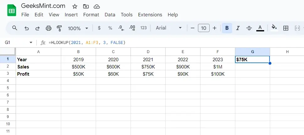
For instance, in the following data, we want to utilize the HLOOKUP() function to find the profit for the year 2021. To do so, firstly, we will select a cell and enter the following formula:
=HLOOKUP(2021, A2:F3, 3, FALSE)
Here:
- “2021” is the value that we need to find.
- “A2:F3” is the range that includes our data and headers.
- “3” refers to the “Profit” row from which we want to retrieve the value.
- “FALSE” is added for an exact match:
Press the “Enter” key and the cell will display “$75K” as the profit for the year 2021:
8. Using LEFT() Function
The LEFT() function extracts or fetches a specified number of characters from the start of a text string.
Formula:
=LEFT(text, num_chars)
The LEFT() function extracts a specified number of characters (num_chars) from the beginning of a text string (text).
Example:
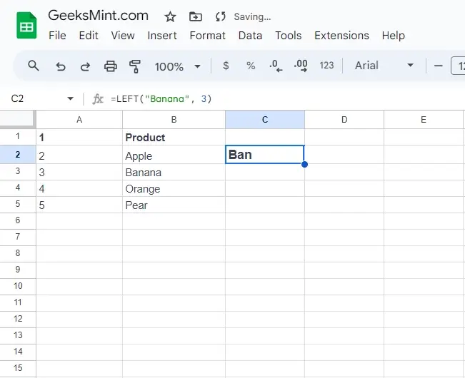
For example, to use the LEFT() function, choose a cell where you want to show the extracted characters. Then, enter the provided formula:
=LEFT("Banana", 3)"
In the above formula, the banana is the one from which we want to extract the first “3” characters:
Conclusion
Now, say no to more tedious, repetitive tasks that drain your day! With these 8 best Excel hacks, you’ll be breezing through your data, crunching numbers, and creating reports in record time.
So, go ahead, put these hacks to good use, save your hours of work, and invest them in some other productive tasks.